Labour-augmenting technical progress

Home > Macro, Solow Model > Labour-augmenting technical progress

Labour-augmenting technical progress

July 18, 2011 mnmecon Leave a comment Go to comments

The basic form of the Solow model gives us a bit of an unsatisfactory conclusion:

1. The economy will grow in terms of output per worker until it reaches a steady state level of output per worker. At steady state level of output per worker, the economy still grows, but it only grows at the rate of labour force growth (which we model as equal to the rate of population growth).

2. Raising the saving rate means you can lift yourself out of steady state and continue to grow for a while until you reach a new steady state. But you will still reach a new steady state point, just at a higher level of output per worker.

So this basically says that all economies will reach a point where they can no longer increase their living standards because output per worker will become constant. Is this realistic? Not really, and if Solow’s model had been left there, probably we wouldn’t be using it so widely.

If the Solow model is to really offer a good framework for thinking about growth, we need some way of explaining how countries can have continuously growing living standards. Solow does it by considering technological progress.

There are various ways that you can incorporate technological progress into the Solow model, but a simple and way of thinking about it is to think of technological progress as being labour augmenting, ie as the state of technology improves, it makes each worker more productive by augmenting their labour. Think about secretaries that used to type letters on typewriters. It may be that now with modern computers that can easily duplicate and edit documents, one secretary now can do the same amount of work as four secretaries could in the days of typewriters (I just made that up by the way). That means that the labour of the secretary has been augmented by the advance of technology, one secretary is now worth four secretaries in the past.

The way to think about this is in terms of ‘effective labour‘.

If you benchmark a particular year where the effective labour of one worker is 1, then you can model technological progress by seeing how technological progress makes effective labour grow. As technology improves, you may find that one worker becomes worth 1.4 effective workers (as benchmarked from the original year). This is a powerful concept, because if technology is improving then it means as your population and labour force grows, you can actually grow your number of ‘effective workers’ faster than the population grows. And going back to the concept of steady state, originally we said that when you are in steady state, your economy grows at the same rate as the labour force grows, so output per capita stays constant….if you are in steady state but with technological progress, then your economy would grow at the same rate as effective workers grow. If effective workers are growing faster than the population, then output per capita will rise and living standards will go up. For an economy, having more effective workers than there are people (because each person is worth more than 1 effective worker due to the technological advances) is a good thing because it means each worker only consumes the amount of one person, but produces the amount of more than one person.

We can look at the algebra of this, its quite similar to the algebra used before in the basic Solow model.

Start with $K_{t+1}= (1-\delta)K_t + sY_t$ .

Now we can define the state of technology as being given by $E_t$ , so we can divide throughout by effective workers, $\frac{E_t}{P_t}$ :

$\frac{K_{t+1}}{E_t P_t}= \frac{(1-\delta)K_t}{E_t P_t} + \frac{sY_t}{E_t P_t}$ .

In the basic model we used small letters to express output and capital per worker, we defined $y_t = \frac{Y_t}{P_t}$ and $k_t = \frac{K_t}{P_t}$ .

Now we are going to think in terms of ‘per effective worker’ so we will put a hat on the small letters: $\hat{y}_t = \frac{Y_t}{E_t P_t}$ and $\hat{k}_t = \frac{K_t}{E_t P_t}$ .

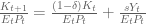
So we have $\frac{K_{t+1}}{E_t P_t}= (1-\delta)\hat{k}_t + s\hat{y}_t$

Now multiply the LHS by $\frac{E_{t+1} P_{t+1}}{E_{t+1} P_{t+1}}$ to get:

$\frac{K_{t+1}}{E_{t+1} P_{t+1}}\frac{E_{t+1} P_{t+1}}{E_t P_t}= (1-\delta)\hat{k}_t + s\hat{y}_t$ which means:

$\hat{k}_{t+1}\frac{E_{t+1} P_{t+1}}{E_t P_t}= (1-\delta)\hat{k}_t + s\hat{y}_t$ .

Now we just need to create a definition for population growth: $\frac{P_{t+1}}{P_t}=(1+n)$ ,

and a definition for growth of technology: $\frac{E_{t+1}}{E_t}=(1+\pi)$ ,

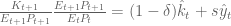
and now we have this expression: $\hat{k}_{t+1}(1+n)(1+\pi)= (1-\delta)\hat{k}_t + s\hat{y}_t$

This is saying that the new per capita capital stock depends on the old per capita stock that is not depreciated, plus the newly accumulated capital stock due to investment. However, the LHS includes population growth and efficiency growth, which is a drag on the per capita stock – the faster population grows, the faster we need to increase capital to keep per efficiency unit of labour stock constant.

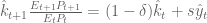
In the end we will tend to a steady state again, where $\hat{k}_{t+1}=\hat{k}_t = \hat{k*}$ .