Cournot competition

In a duopoly, the residual demand curve faced by one firm is the market demand curve minus the supply of the rival firm: .

In the simple model I’m using for these examples, the market demand is Q = 500 – P and the firm (both firms in this duopoly case) have no fixed costs and a constant marginal cost of 150. So if the firms are firm A and firm B, then the residual demand curves for each firm are: and .

This means the inverse residual demand curves for each firm are .

We established that the best response curve for firm A is

What about firm B? Again the inverse residual demand curve for firm B is , so the total revenue is .

The marginal revenue is .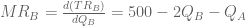

The profit maximising quantity of output is where MR = MC, so .

This is the best response function for firm B, so we can add this to the best response curve graph.

Previously we considered what the best response would be for firm A if firm B produced 200: firm A would be best to produce 75.

But if firm A was to produce 75, then it is no longer optimal for firm B to produce 200. If firm A produces 75, then the best response for firm B is to produce .

So if firm B thinks that firm A is basing its decision on B producing 200, then firm A is going to produce 75. Knowing this, firm B will be better to actually produce 137.5.

But if firm B was to produce 137.5, then it is no longer optimal for firm A to produce 75! If B produces 137.5, then A should produce .

This kind of decision making and guesswork can go on and on, this is strategic thinking. You are trying to guess what your rival will do, and choosing the optimal response to that, but you are taking into account the fact that your rival is basing its decision on what it thinks your firm will do, and choosing its optimal response to that.

Where will it end? The answer is when you reach a Nash equilibrium, which is a position where neither firm wants to change its decision based on the output decision of the other. So you need to find a point where both firms are happy to ‘stick’ based on the output they expect from the other.

In this duopoly model, where both firms are identical and are competing with each other based on the quantity of output they produce, the Nash equilibrium we are looking for is called a Cournot equilibrium. We are assuming here that neither firm knows the output decision of the other when it makes its own decision – it is just guessing, and both firms are making their decision simultaneously, one does not announce its output decision before the other.

Notice how on the graphs, each time the firms change their decision based on what they think the other will do, their output decisions approach the point where the two best response curves intersect. This is a clue as to how to find the answer – it is at the intersection point of the curves. So you can solve this by setting the best response curves equal to each other.

We had the best response curve for firm A: , and the best response curve for firm B: , so we can just substitute one into the other:

. So firm A will produce 116.667.

Substituting this back into the best response function for firm B, . So firm B will also produce 116.667.

Now we have reached a Cournot equilibrium. If firm A produces 116.667 then firm B’s best response is to also produce 116.667. And if firm B produces 116.667 then firm A’s best response is to also produce 116.667. No other combination will be on the best response curves of both firms, so this is the Cournot equilibrium.

In the monopoly form of the model, the firm was producing output of 175, selling at a price of 325. It was making profits of 30625 and had a Lerner Index of 0.538.

Now in the Cournot duopoly, each firm produces output of 116.667 which means the total market output is 233.333, and the market price is 500-233.333 = 266.667. So the price to consumers has fallen. Each firm is making profits of 266.667(116.667) – 150(116.667) = 13611.11, and has a Lerner Index of 0.438 showing that the amount of market power has dropped.

What would happen if the firms were not identical and had different marginal costs? Consider the case where the new entrant, firm B, was more efficient than the incumbent firm, firm A, and whereas firm A had a marginal cost of 150, firm B had a marginal cost of 120.

This time, firm B’s best response curve would be different. The marginal revenue is 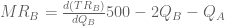, so for firm B to produce at the profit maximising point where MR = MC, then .

Firm A’s best response curve is unchanged as the marginal cost is still 150 so setting MR = MC will give us the same result. But this time, to find the Cournot equilibrium we solve these simultaneous equations:
Best response curve for firm A: , and best response curve for firm B: , so we substitute one into the other:

. This time it is best for firm A to produce a lower amount, 106.667.

And if firm A produces 106.667 then firm B should produce . This time it is best for firm A to produce a higher amount, 136.667.

Firm B can produce more than firm A in the new Cournot equilibrium because it has a lower marginal cost – it is a more competitive producer.

With firm A producing 106.667 and firm B producing 136.667 the total market output is 243.333 and so the market price is 500-243.333 = 256.667. Firm A will produce profits of 11377.778 and have a Lerner index of 0.416 and firm B will produce profits of 18677.778 and have a Lerner index of 0.532.